In this post I will discuss my implementation of a support vector machine (SVM) based binary classification system for spam filtering. In future posts I plan to compare the performance of this technique with other classification algorithms such as logistic regression and neural networks. Following on from exercise six of the Stanford University Machine Learning course, I will be using the SpamAssassin public mail corpus to train, validate and test my classification system. The SpamAssassin emails can be found here: https://spamassassin.apache.org/publiccorpus/. The data set consists of 6,046 emails of which 4,150 have been classified as non-spam and 1,896 as spam.
My goal for this analysis is multifold. Firstly, to create a robust SVM (linear kernel) classification spam filter using the LIBSVM package (https://www.csie.ntu.edu.tw/~cjlin/libsvm/). Secondly, to determine the performance of the classification system using a range of different metrics including learning curves, true positive rates, false positive rates, recalls, precisions, F1 scores, receiver operating characteristic (ROC) curves and area under curve (AUC) values. Thirdly, to use the SVM performance as a standard of which to compare the performance of other classification algorithms.
Feature creation
An important step in any machine learning implementation is the creation of useful features to train and test the algorithm. The method I use here is to generate a vocabulary of unique words from the emails that are known to be spam. Each email in the training set then goes through a detection algorithm that determines if these unique words are used in each email. The results of this step are then used as the features to train the network. The features are split into training, cross-validation and testing subsets with a 80-10-10 ratio. The determination of what model parameters to use will be based on tests performed on the cross-validation data. The final step will be to apply the model to the test data to determine the overall performance.
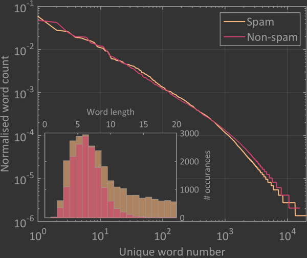
The steps to create the vocabulary list have been adapted from an algorithm utilised in the Machine Learning course from Stanford University. Briefly, the algorithm removes all header information, forces lowercase, strips all HTML, punctuation and non-alphanumeric characters, converts all URLs, numbers and email addresses to pre-defined strings, stems all possible words, removes words less than 1 and greater than 20 characters in length, and finally identifies all unique words and sorts them according to a descending order of usage. Using this method 26,901 unique words were detected in the spam emails. The same algorithm applied to the same number of non-spam emails yields 15,926 unique words, which is an interesting observation in itself.
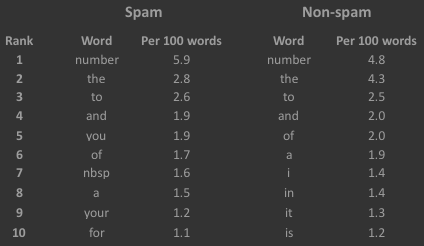
The ten most common words from the two categories of emails are presented above. The seventh entry ‘nbsp’ in the spam list is an interesting one. This is leftover from a ‘non-breakable space’ character that is used in word processing and typesetting. I left it in the spam vocabulary upon realising that it is quite far down the non-spam list (610th entry), which may indicate that it is a good feature to detect spam.
Before creating my SVM spam filter I found it interesting to compare the spam and non-spam vocabularies even though only the spam vocabulary will be used in the model. Plotting their distributions after normalising to their respective sums on top of each other shows that they follow basically the same trend. Interestingly, when you do a histogram of the word lengths in each vocabulary, we find that the spam emails have many more long words than the non-spam. There are very few words above 10 characters long in the non-spam emails whereas the spam emails have a significant population of 20 character words. This result suggests that the average length of the words could likely be used as a feature.
In total the spam vocabulary contains 26,901 unique words that can be used as features in the SVM classification algorithm. Near the end of this list are words that were only detected once or two in all of the 1,896 emails used to create the vocabulary. I suspect that these words are probably worthless and merely increase the computational expense without adding any predictive value. The first test will be to determine how many of the features are actually useful so that the computational time can be reduced.
Determining the number of useful features
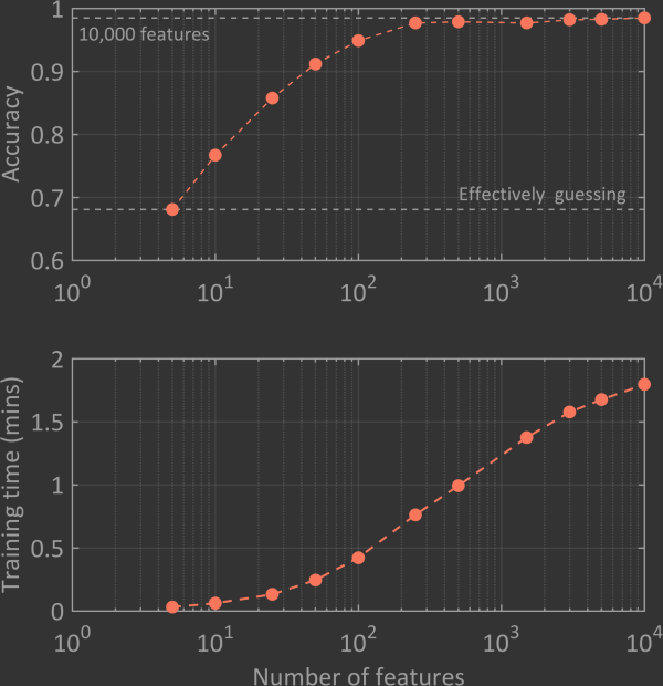
To get an idea for how many features of the possible 26,901 are necessary, I performed the following simple analysis. Firstly, I varied the number of training features fed to the SVM and monitored the achieved classification accuracy when the model was applied to the cross-validation set. As the number of training features increased from 5 up to about 100, the accuracy increased from just below 0.70 up to about 0.95. As the number of features increases passed a few hundred the accuracy plateaus at the 0.98 level. This plateau shows that arbitrarily increasing the number of features will not significantly increase the accuracy of the classification algorithm. Secondly, I monitored the time it took to train the data set for the different range of features. Unlike the accuracy, which plateaus at some point, the training time continues to grow with increasing feature number. These results show that there would be no gain from using all 26,901 features in my spam filtering system. Therefore, in the following I will only be using the 10,000 most common words from the total vocabulary.
Principal component analysis
The above discussion about the number of useful features highlights how model complexity can be significantly reduced while conserving predictive capabilities. A related concept is called principal component analysis (PCA – https://en.wikipedia.org/wiki/Principal_component_analysis), which is a method that can reduce the number of features while retaining most of the information. This is achieved by replacing sets of correlated features with sets of uncorrelated features. For example, in spam emails two particular words might often be used in combination. In this case, instead of having one feature per word it might only necessary to have one feature that describes them both. Utilising PCA intrinsically means that some data will be lost and the predictive capabilities of the SVM will be reduced. In reality, there is a tradeoff between how much data compression you need and the predictive accuracy that you desire.
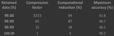
In the table above the achievable feature reduction, associated computational savings and attainable accuracies are summarise for different values of the retained data. The accuracies were found by testing against the cross-validation data. As expected, as the amount of retained data is reduced the compression factor significantly increases. In the case of retaining 99% of the data, the 10,000 features are able to be reduced to only three features! Unfortunately, in this case the predictive accuracy decreases from 98.2% to 94.2%, which highlights the compromise that has to be made. The choice of whether you retain more or less data depends on the overall goal. Since one of my main goals is to achieve a high prediction accuracy, I will utilise PCA with 99.99% retainment of the data. This means minor information loss with a 40% decrease in computational time. Note that since all of the features are of a similar value, consisting of only 1s or 0s that indicate whether a particular word is present in the email, I did not perform feature normalisation on the data before implementing PCA.
Classification capabilities
The capabilities of a classification algorithm can be diagnosed in a number of ways. The accuracy of the model, as used above, is the most obvious metric. However, using accuracy by itself can be dangerous since in some circumstances a model with no predictive ability can actually reach high values. The description of some common metrics are:
Accuracy: proportion of correctly identified spam and non-spam emails.
Recall: proportion of spam emails that are identified as spam.
Precision: proportion of identified spam emails that are actually spam.
F1 score: harmonic mean of the recall and precision.
True positive rate (TPR): the proportion of spam emails that are identified as spam.
False positive rate (FPR): the proportion of non-spam emails that are identified as spam.
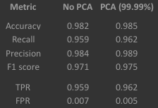
Above are the values of each metric after testing on the cross-validation data set when PCA is and isn’t utilised. The values are extremely close between the two data sets, showing that very little data was lost during the PCA process. Also, it is clear that the classification system works quite well with high values for all metrics except the FPR but this is good since a small value is desired here.
Overfitting or underfitting?
While the above metrics give an idea about the performance of the classification system, they don’t include information about whether the model is too complex or too simple for the data. An overly complex model can result in what is commonly called overfitting where the model fits the training data extremely well but may not be able to correctly classify new data. A model that is too simple can result in underfitting where the model doesn’t fit the data at all and also has no predictive capabilities for new data. In general, overfitting seems to be a more common problem since the inclination for most people is to do whatever you can to improve the above metrics. While this might be a good method to enhance your model, it can also easily result in overfitting. A common method to limit this possibility is to implement what is called regularisation. This is a difficult subject to comprehensively explain (even for academic experts) but in practical terms for the case of regression it penalises large fitting parameters, which results in smoother fits to the data and less complicated models. For SVMs regularisation is a method to decided whether you want to more emphasis on correctly classifying all data points or on creating a more realistic looking classification boundary.
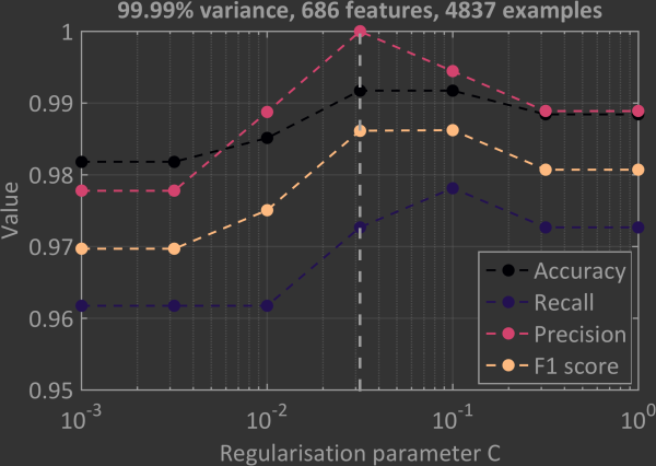
In SVMs regularisation is controlled by the parameter C. You want to find a value of C where the model neither over- nor underfits. Using overly large values of C tends to result in overfitting while using overly small values of C tends to result in underfitting. The most common method to determine the best value of C is a brute force trial and error approach. In the above plot the C values were scanned through the range 10-3 – 10+1 while the diagnostic parameters mentioned above were monitored. In this test the maximum number of features and examples were used to train the SVM. The line at 10-1.5 is the value of C chosen for the next few steps since it gives close to the maximum value for each of the parameters. Values of C above 10-2 and below 10-1 would probably be good choices too since all parameters are quite high within that interval. Outside of this range the parameters do not seem to change, which may indicate regions of under- and overfitting.
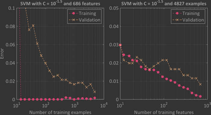
Importantly, implementing regularisation doesn’t guarantee that overfitting or underfitting isn’t taking place and further tests should be performed to double check. One method is to create so-called learning curves, which are he result of training the model over a range of either training examples or features while the training and cross-validation predictive errors are monitored. The above graph presents such SVM learning curves with C = 10-1.5. The results shown in the left panel are as a function of the number of training examples and in the right panel as a function of the number of features. Both graphs suggest that overfitting is not occurring since the validation error continues to decrease as both x-axes are increased. Underfitting also does not seem to be an issue since in the left panel the validation error converges to the training error at a low value. If underfitting were present this convergence would occur at a high training error.
Decision threshold
This binary classification SVM outputs a probability of whether an email is spam or not. A high probability suggests that the email is spam while a lower probability suggests it is a normal email. The decision of what is a ‘high’ probability is determined by the threshold parameter. Effectively, if the output probability is greater than or equal this threshold then the email is considered spam. The default value for this parameter is normally 0.5, and indeed this is the value that was used for all of the results presented so far. However, this doesn’t have to be the case as it can be varied anywhere between 0 – 1. Varying the threshold while monitoring the true positive rate (TPR) and the false positive rate (FPR) leads to so-called receiver operating characteristic (ROC) curve (https://en.wikipedia.org/wiki/Receiver_operating_characteristic), which is one of the best ways to characterise binary classification systems. Each point on an ROC curve corresponds to the TPR and FPR determined when using a particular threshold value.
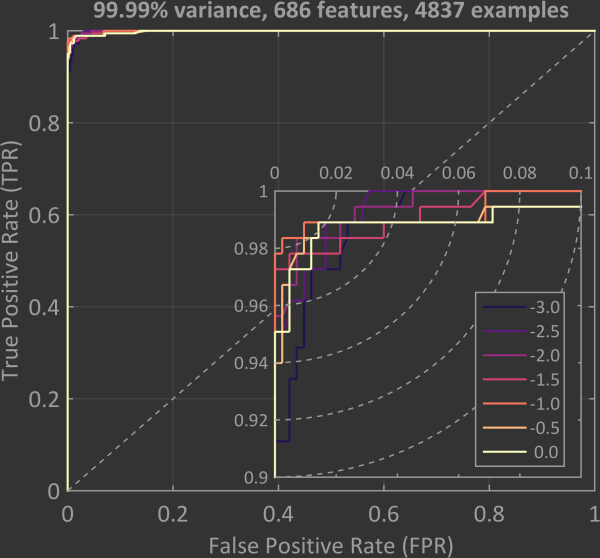
An ROC curve is plotted above for training the SVM binary classifier with PCA and a variance of 99.99% and testing the model with the cross-validation data set. The dashed line along the diagonal represents a binary classification algorithm that has no predictive ability. Any curve that is above this line represents a model that is able to classify with a probability above chance. The curve of an ideal model would increase along the y-axis at x = 0 until making a right angle turn at x = 0, y = 1. The curve would then follow along the positive x direction at y = 1. The area under such an ideal curve would be equal to one. Such an idealised curve doesn’t exist in reality but as can be seen in the plot below the ROC curves are quite close over a wide range of C values. The inset shows a zoomed in view of the top left corner and highlights just how close to ideal the results are.
The best AUC value found for the cross-validation data is 0.9993 at C = 10-2. The highest level of accuracy was found to be 0.9934 at C = 10-1 and a threshold value between 0.42 – 0.64. Interestingly, this is also where the highest F1 score of 0.9890 was achieved. The fact that the best results were found for values of C between 10-2 and 10-1 is consistent with the earlier tests.
Summary
The final step is to apply the model to the test data set. We do this because we have used the cross-validation data set to modify and improve the model. Effectively this means that we have been performing another type of fitting to the data. It is therefore a good idea to determine the robustness of the model using data that the model is yet to have seen. I guess you will have to take me word for it that this is the case. Since I feel like the best results for the cross-validation data were found at C = 10-1, I have selected this as the regularisation parameter for the model. Since the cross-validation results gave a wide range of potential best threshold settings, I allowed myself the luxury of picking the threshold value between 0.42 and 0.64 that gave the best testing results. This value happened to be 0.6. Using these parameters the SVM spam filter achieved a final accuracy of 0.9851, a recall of 0.9671, a precision of 0.9904 and an F1 score of 0.9786.
Now that a robust and accuracy spam filter has been developed using an SVM with a linear kernel, I plan to use its performance as a standard to test other classification methods against. Next up, I will implement a Gaussian kernel SVM and a neural network to see if using these methods can improve classification.
Mick
2016/09/16
